Total Clients cumulative Total Referrals cumulative and Top 3 Service Categories see example below. In the Series values.
Select From Drop Down And Pull Data From Different Sheet In Microsoft Excel 2016
3 Click Add button to add the data range into the All references list box.

How to create a roll up tab in excel. Make a project table. And formua-fill that sideways for the required number of columns say to column M etc then select that range say A1M1 and formula-fill downwards for the correct number of rows say 150. An example of a 3D SUM formula is SUMSheet1Sheet5A1 This formula will return the sum of the values in the cell A1 of all those 5 sheets from sheet1 to sheet5 assuming there are 10 sheets like sheet1sheet2 sheet3 sheet4 and sheet5.
Select the Developer Check box. Then go to the Design tab under Chart Tools and click the Move Chart button. Create 12 sheets for Every Month in a workbook.
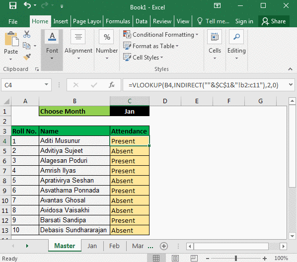
Heres a simple guide to do it. Select the range of cells in your spreadsheet that you want to convert to a table and open the Home tab. If you plan to track attendance for a year you will need to create each months sheet in Excel.
2 Click to select the range of each sheet you want to collect. Create a Basic Table. Text box in the Edit Series dialog box replace the default table range with the dynamic data named range.
Enter the initial date in the first cell. Select the rows you want to fold and go to Data tab. After that draw a rectangle in the excel worksheet to insert a ScrollBar.
A hover box at least thats what Ive always read them named are the boxes that pop up when you point your mouse on something and hold it for a second or two a message box pops up and gives you a description of what you are pointing at. If you wanted to create a Total sheet and have a table in it that sums up each of the tables in the Jan to Dec sheets then you could use this formula and copy it across the whole table. Fold Rows in Excel.
Click the Format as Table drop-down box in the ribbon and choose the style youd like to use. Form Validation criteria choose the List option. To auto generate a series of days weekdays months or years with a specific step this is what you need to do.
If you want to make it more concise and intuitive to find the specific data you can fold the rows or columns by adding a data group. Use Insert - Pivot Table. On the Design tab click Select Data.
If you are looking to add the data from multiple worksheets in an Excel workbook you can use 3D SUM for the same. On the Settings tab select List from the Allow drop-down list see drop-down lists are everywhere. Add Columns for each date in each months sheet.
Create tables from your Microsoft Excel worksheets. Select the source tab where excel will ask for the database cell to appear in the drop-down list. In the Consolidate dialog do as these.
Click the Manage icon on the Power Pivot tab in the Ribbon. In the pop-up menu choose Series the last item. Now select the cell into which you want to add a drop-down list and click the Data tab.
In this article we will learn how to do so. The Data Validation dialog box displays. Data Validation Dialogue box appears as follows.
Alternately you can enter in A1 of the Summary the formula. If you will move the rectangle spread more horizontally then the Horizontal Scroll. SUM15B3 this is called the 3D Sum You just need to type the first sheet name then select the cell in the last sheet this will return the sum of all the number in inbetween tab.
Steps to create a Gantt chart in Excel. Click on the chart to activate the Chart Tools contextual tabs. Click on the Insert tab select the bar charts group.
Many instances of Excel 2013 and 2016 do not have this tab. Click on Insert then click the SCROLLBAR control to insert the new list box in excels worksheet. In the opening Add-Ins dialog box check the Analysis ToolPak in the Add-Ins available box and click the OK button.
You could also give the chart a different name at this point. If the color of the table isnt a concern you can simply insert a basic table. The first table will be the WAServes Snapshot table lists four key metrics.
New Sheet and Object in Select New Sheet. You can create an Attendance tracker in Excel easily. An Excel spreadsheet can be very large containing a lot of information.
Select range of start date B1. Click on the Data Tab. Click on the Excel Ribbon then select the Developer tab.
Create a Running Balance using the OFFSET Function The OFFSET function allows you to create a reference by specifying the number of rows and columns offset from a particular reference. In the Excel Options dialog box click the Add-Ins in the left bar Keep Excel Add-Ins selected in the Manage box and then click the Go button. In the Data Tools section of the Data tab click the Data Validation button.
To create Drop Down list in Excel follow the below steps as shown below. You too can create a Microsoft Word document for your Organizations Weekly Roll-up Report. In the Select Data Source dialog box select the first data series and click.
1 Select one operation you want to do after combine the data in Function drop down list. Now you get back to the main interface of Excel. In the Create PivotTable dialog choose the box for Add This Data to the Data Model.
I was wondering if I can make a cell have a hover box. Here is the PivotTable Fields before you create the hierarchy. Each task is mentioned in a separate row with the respective start date and tenure number of days required to complete that task.
Make an Excel bar chart. Select that cell right-click the fill handle drag it through as many cells as needed and then release. The Move Chart dialog will open and youll see two options.
There are two fairly simple solutions for creating a robust running balance that dont break when you insert delete or move rows.
How To Modify The Worksheet Tab In Excel Video Lesson Transcript Study Com

Change Worksheet Tab Color In Excel Instructions
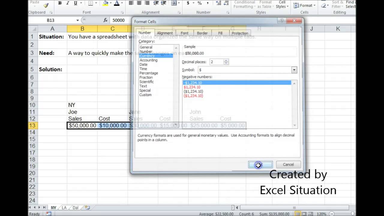
Excel Making The Same Changes On Multiple Tabs Youtube

Create Summary Sheet Sort Data Automatically Youtube
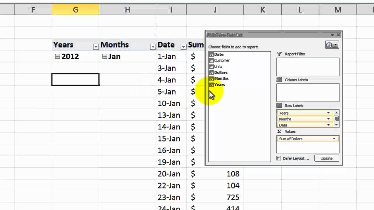
How To Create A Roll Up By Month Filter In An Excel Pivot Table Youtube