In the pivot table shown there are three fields Name Date and Sales. Here is a demo of the types of filters available in a Pivot Table.
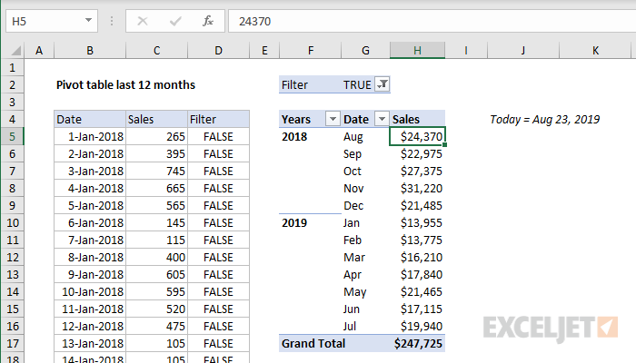
Pivot Table Pivot Table Last 12 Months Exceljet
Click the arrow next to the time level shown and pick the one you want.
How to create a roll up by month filter in an excel pivot table. Figure 2 Setting up the Data. We will create a Pivot Table with the Data in figure 2. By default the Months option is selected.
Lets look at these filters one by one. This filter allows you to drill down into a subset of the overall dataset. Note that we have put the data in a table form by doing the following.
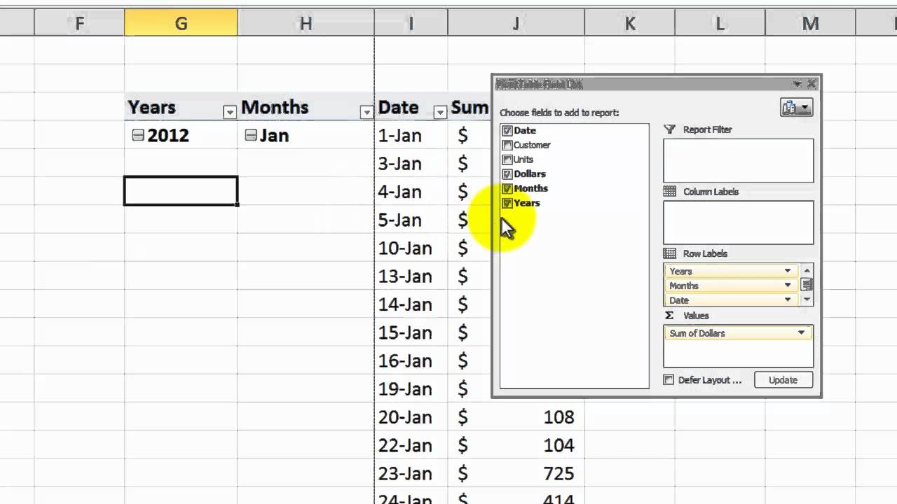
Excel may have created a Year andor Month field automatically. When you click on the Group option it will show us below the window. By default a pivot table is set up to.
Or in Excel 2010 you can also click on the Group Field icon on the contextual Pivot Table toolbar. In the Between dialog box type a start and end date or select them from the pop up calendars. With your Timeline in place youre ready to filter by a time period in one of four time levels years quarters months or days.
Below is my data. On the Design tab click Select Data. Again as soon as a new filter is applied the old filter is removed.
In this window we can see it has picked automatic dates at starting at ending at dates. In column A I have the date for each record and in column C I use an IF function to compare todays date returned from your computers clock using the TODAY function in cell F2 to the date in column A to see if it falls within the last 12 months. Use a Timeline to filter by time period.
In the Create PivotTable dialog box specify the destination range to place the pivot table and click the OK button. 4 Now select any of the days and right-click. In the example shown the pivot table is uses the Date field to automatically group sales data by month.
I have attached an example of the data but I only want to show the last 12 months of. Right-click on any of the cells of the Date column and choose the Group option. Please do as follows.
Click on the chart to activate the Chart Tools contextual tabs. Filter the most recent rolling 12 months from a table in Power Query Step 1. Click the drop down arrow on the Row Labels heading.
First highlight one of the cells of the Pivot table containing data. On the Analyze tab click Group Field in the Group option. Figure 1- How to Group Pivot Table Data by Month.
To build a pivot table to summarize data by month you can use the date grouping feature. We clicked on anywhere on the table click on the Insert tab and click on Table as shown in figure 3. Text box in the Edit Series dialog box replace the default table range with the dynamic data named range.
First select one of the Years. Drag a date field into the Row or Columns area in the PivotTable Fields task pane. For example lets add Quarters to our pivot table.
Group date by month quarter or year in pivot table. First thing we need to do is grab the data. In the same way.
Creating Excel Slicers for Rolling Periods. Select a date field cell in the pivot table that you want to group. Insert the pivot table first like the below one.
Click in a pivot table. Types of Filters in a Pivot Table. Select the source data and click Insert PivotTable.
Select the data range you need and click Insert PivotTable. Finally choose the Show Details option from the appearing list. There is a Group function in pivot table you can apply it to group data as your need.
In the Insert Timeline dialog box check the date fields you want and click OK. When drag and drop the date field as the first-row label you can filter date range in the pivot table easily. Either of these methods brings up a Grouping date dialog box.
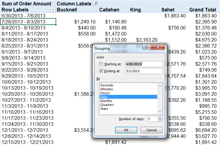
Choose the Group By option as. We will click on. In the GROUPING dialog box select DAYS and 7 in the NUMBER OF DAYS drop-down list.
Setting up the Data. In Excel 2013 and later there is a Whole Days option. In the Series values.
In the resulting Create PivotTable dialog box we tell Excel to place the report on the desired worksheet and click OK. Create a Pivot table to show 12 months rolling data. When your field contains date information the date version of the Grouping dialog box appears.
Figure 3- Putting the data in a Table. To build the basic PivotTable we select any cell in the data table and then use the Insert PivotTable ribbon icon. From the pop-up menu select GROUP.
For this you add or remove check marks in the list of pivot items for the field. Now only the sales from the first 3 months are shown. In the Select Data Source dialog box select the first data series and click.
Select the Field name from the drop down list of Row Labels fields. Add a Manual Filter. For example if you have retail sales data you can analyze data for each region by selecting one or more than regions yes it allows multiple selections as well.
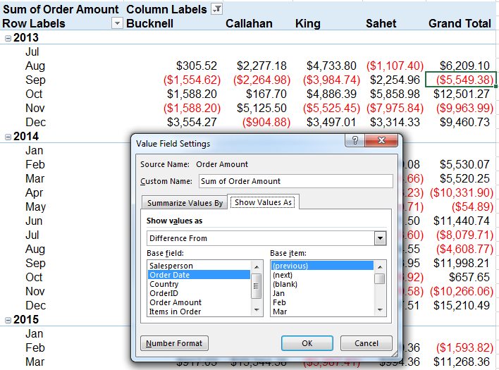
To do this we have to select any cell inside of our pivot table here and go over to the pivot table field list and going to remove Industry from the rows removing Count of Age Category from the values area and we are going to take the Function that is in our filters area to rows area and so now we can see that we have a list of our filter criteria if we look over here in our filter drop. When we click OK we get a breakdown of sales by year and quarter. To group by month andor year in a pivot table.
Then right-click and choose Group. How to Create a Roll up by Month Filter in an Excel Pivot Table - YouTube. Change the Pivot Table Filter Options.
After this right-click the highlighted cell. Finally well try a Manual Filter. Your Pivot Table will be created automatically.
Then we insert the Date field into the Rows area and the Amount field into the Values area. You can either right-click on the dates. In other words I want to roll up the dates and view it by month and by year.
Right-click the cell and select Group from the drop-down menu. Click Date Filters then click Between. 3 Click DATA to insert it in the VALUES quadrant of the Pivot Table and click DAYS to insert it in the ROWS quadrant.
To do this I clicked in the table and. Power Query From Table Confirm the range if required Changed the query name to Rolling12. You have choices to group by Seconds Minutes.
Now just click Quarters to add them to Years. Instead of the Show Details command theres a lot faster solution to achieve the drill-down.

The Excel Pivottable Group By Month Pryor Learning Solutions
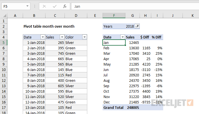
Pivot Table Pivot Table Month Over Month Exceljet
The Excel Pivottable Group By Month Pryor Learning Solutions
How To Create A Roll Up By Month Filter In An Excel Pivot Table Youtube
The Excel Pivottable Group By Month Pryor Learning Solutions